上海频道做网站怎么样西安网站建设公司十强

完整代码见 Github：https://github.com/ChaoQiezi/read_fy3d_tshs，由于代码中注释较为详细，因此博客中部分操作一笔带过。

01 FY3D的HDF转TIFF

1.1 数据集说明

FY3D TSHS数据集是二级产品(TSHS即MWTS/MWHS 融合大气温湿度廓线/稳定度指数/位势高度产品)；
文件格式为HDF5；
空间分辨率为33KM（星下点）；
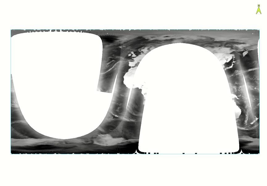
范围为全球区域；(FY3D为极轨卫星，因此对于得到的单个数据集并没有完全覆盖全球区域)，类似下方（其余地区均未扫描到）：

提取数据涉及的多个数据集：

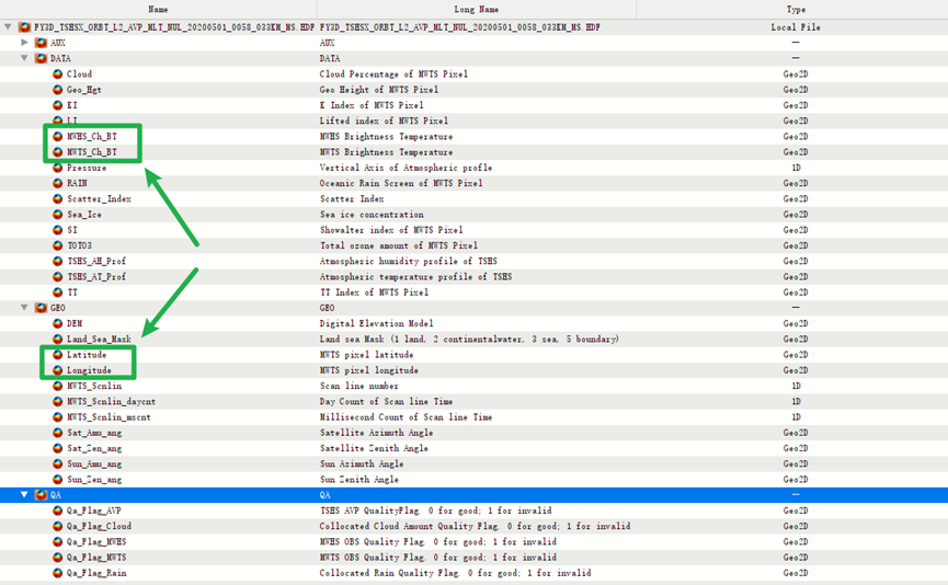
位于DATA/MWHS_Ch_BT和DATA/MWTS_Ch_BT 路径下的两个数据集分别为MWTS 通道亮温和MWHS 通道亮温，这是需要提取的数据集；
另外位于GEO/Latitude 和GEO/Longitude 路径下的两个数据集分别经纬度数据集，用于确定像元的地理位置以便后续进行重投影；

1.1.1 MWTS 通道亮温和MWHS 通道亮温数据集的说明

这是关于数据集的基本属性说明：

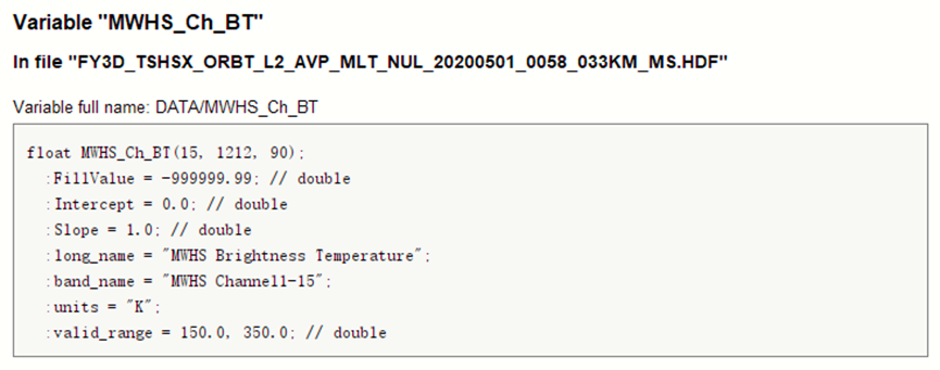
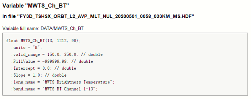
在产品说明书中关于数据集的说明如下：

可以发现，其共有三个维度，譬如MWHS_Ch_BT数据集的Shape为(15, 1212, 90)，其表示极轨卫星的传感器15个通道(即波段数)在每条扫描线总共 90 个观测像元的MWHS亮温值，此处扫描线共有1212个。对于MWTS数据集类似格式。（这意味着三个维度中并没有空间上的关系）

1.1.2 经纬度数据集的说明

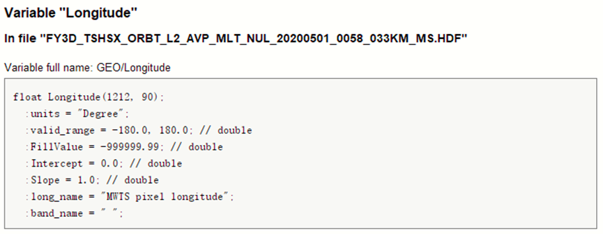
这是官方产品说明对于经纬度数据集的介绍：

可以发现，经纬度数据集的Shape均为(1212, 90)，这正好对应前文提及的两个数据集的所有像元（除去波段数），其表示每条1212条扫描线上的90个观测像元的经纬度。

1.2 读取HDF5文件数据集

def read_h5(hdf_path, ds_path, scale=True):"""读取指定数据集并进行预处理:param hdf_path: 数据集所在HDF文件的绝对路径:param ds_path: 数据集在HDF文件内的路径:return: 返回处理好的数据集"""with h5py.File(hdf_path) as f:# 读取目标数据集属矩阵和相关属性ds = f[ds_path]ds_values = np.float32(ds[:])  # 获取数据集valid_range = ds.attrs['valid_range']  # 获取有效范围slope = ds.attrs['Slope'][0]  # 获取斜率(类似scale_factor)intercept = ds.attrs['Intercept'][0]  # 获取截距(类似add_offset)""""原始数据集可能存在缩放(可能是为存储空间全部存为整数(需要通过斜率和截距再还原为原来的值,或者是需要进行单位换算甚至物理量的计算例如最常见的DN值转大气层表观反射率等(这多出现于一级产品的辐射定标, 但二级产品可能因为单位换算等也可能出现));如果原始数据集不存在缩放, 那么Slope属性和Intercept属性分别为1和0;这里为了确保所有迭代的HDF文件的数据集均正常得到, 这里依旧进行slope和intercept的读取和计算(尽管可能冗余)"""# 目标数据集的预处理(无效值, 范围限定等)ds_values[(ds_values < valid_range[0]) | (ds_values > valid_range[1])] = np.nanif scale:ds_values = ds_values * slope + intercept  # 还原缩放"""Note: 这里之所以选择是否进行缩放, 原因为经纬度数据集中的slope为1, intercept也为1, 但是进行缩放后超出地理范围1°即出现了90.928对于纬度。其它类似, 因此认为这里可能存在问题如果进行缩放, 所以对于经纬度数据集这里不进行缩放"""return ds_values

上述代码用于读取指定HDF5文件的指定数据集的数组/矩阵，scale参数用于是否对数据集进行slope和intercept线性转换。

1.3 重组和重投影

这一部分是整个数据处理的核心。

1.3.1 重组

def reform_ds(ds, lon, lat, reform_range=None):"""重组数组:param ds: 目标数据集(三维):param lon: 对应目标数据集的经度数据集():param lat: 对应目标数据集的纬度数据集(二维):param reform_range: 重组范围, (lon_min, lat_max, lon_max, lat_min), 若无则使用全部数据:return: 以元组形式依次返回: 重组好的目标数据集, 经度数据集, 纬度数据集(均为二维数组)"""# 裁选指定地理范围的数据集if reform_range:lon_min, lat_max, lon_max, lat_min = reform_rangex, y = np.where((lon > lon_min) & (lon < lon_max) & (lat > lat_min) & (lat < lat_max))ds = ds[:, x, y]lon = lon[x, y]lat = lat[x, y]else:ds = ds.reshape(ds.shape[0], -1)lon = lon.flatten()lat = lat.flatten()# 无效值去除(去除地理位置为无效值的元素)valid_pos = ~np.isnan(lat) & ~np.isnan(lon)ds = ds[:, valid_pos]lon = lon[valid_pos]lat = lat[valid_pos]# 重组数组的初始化bands = []for band in ds:reform_ds_size = np.int32(np.sqrt(band.size))  # int向下取整band = band[:reform_ds_size ** 2].reshape(reform_ds_size, reform_ds_size)bands.append(band)else:lon = lon[:reform_ds_size ** 2].reshape(reform_ds_size, reform_ds_size)lat = lat[:reform_ds_size ** 2].reshape(reform_ds_size, reform_ds_size)bands = np.array(bands)return bands, lon, lat

这部分是对原始数据集(此处理中待重组数据集shape为(15, 1212, 90))进行重组。
重组原理即基于经纬度数据集，依据裁剪范围将满足地理范围内的所有有效像元一维化，然后重新reshape为二维数组，数组行列数均为原维度的平方根。

1.3.2 重投影

def data_glt(out_path, src_ds, src_x, src_y, out_res, zoom_scale=6, glt_range=None, windows_size=9):"""基于经纬度数据集对目标数据集进行GLT校正/重投影(WGS84), 并输出为TIFF文件:param out_path: 输出tiff文件的路径:param src_ds: 目标数据集:param src_x: 对应的横轴坐标系(对应地理坐标系的经度数据集):param src_y: 对应的纵轴坐标系(对应地理坐标系的纬度数据集):param out_res: 输出分辨率(单位: 度/°):param zoom_scale::return: None"""if glt_range:# lon_min, lat_max, lon_max, lat_min = -180.0, 90.0, 180.0, -90.0lon_min, lat_max, lon_max, lat_min = glt_rangeelse:lon_min, lat_max, lon_max, lat_min = np.nanmin(src_x), np.nanmax(src_y), \np.nanmax(src_x), np.nanmin(src_y)zoom_lon = zoom(src_x, (zoom_scale, zoom_scale), order=0)  # 0为最近邻插值zoom_lat = zoom(src_y, (zoom_scale, zoom_scale), order=0)# # 确保插值结果正常# zoom_lon[(zoom_lon < -180) | (zoom_lon > 180)] = np.nan# zoom_lat[(zoom_lat < -90) | (zoom_lat > 90)] = np.nanglt_cols = np.ceil((lon_max - lon_min) / out_res).astype(int)glt_rows = np.ceil((lat_max - lat_min) / out_res).astype(int)deal_bands = []for src_ds_band in src_ds:glt_ds = np.full((glt_rows, glt_cols), np.nan)glt_lon = np.full((glt_rows, glt_cols), np.nan)glt_lat = np.full((glt_rows, glt_cols), np.nan)geo_x_ix, geo_y_ix = np.floor((zoom_lon - lon_min) / out_res).astype(int), \np.floor((lat_max - zoom_lat) / out_res).astype(int)glt_lon[geo_y_ix, geo_x_ix] = zoom_longlt_lat[geo_y_ix, geo_x_ix] = zoom_latglt_x_ix, glt_y_ix = np.floor((src_x - lon_min) / out_res).astype(int), \np.floor((lat_max - src_y) / out_res).astype(int)glt_ds[glt_y_ix, glt_x_ix] = src_ds_band# write_tiff('H:\\Datasets\\Objects\\ReadFY3D\\Output\\py_lon.tiff', [glt_lon],#            [lon_min, out_res, 0, lat_max, 0, -out_res])# write_tiff('H:\\Datasets\\Objects\\ReadFY3D\\Output\\py_lat.tiff', [glt_lat],#            [lon_min, out_res, 0, lat_max, 0, -out_res])# # 插值# interpolation_ds = np.full_like(glt_ds, fill_value=np.nan)# jump_size = windows_size // 2# for row_ix in range(jump_size, glt_rows - jump_size):#     for col_ix in range(jump_size, glt_cols - jump_size):#         if ~np.isnan(glt_ds[row_ix, col_ix]):#             interpolation_ds[row_ix, col_ix] = glt_ds[row_ix, col_ix]#             continue#         # 定义当前窗口的边界#         row_start = row_ix - jump_size#         row_end = row_ix + jump_size + 1  # +1 因为切片不包含结束索引#         col_start = col_ix - jump_size#         col_end = col_ix + jump_size + 1#         rows, cols = np.ogrid[row_start:row_end, col_start:col_end]#         distances = np.sqrt((rows - row_ix) ** 2 + (cols - col_ix) ** 2)#         window_ds = glt_ds[(row_ix - jump_size):(row_ix + jump_size + 1),#                     (col_ix - jump_size):(col_ix + jump_size + 1)]#         if np.sum(~np.isnan(window_ds)) == 0:#             continue#         distances_sort_pos = np.argsort(distances.flatten())#         window_ds_sort = window_ds[np.unravel_index(distances_sort_pos, distances.shape)]#         interpolation_ds[row_ix, col_ix] = window_ds_sort[~np.isnan(window_ds_sort)][0]deal_bands.append(glt_ds)# print('处理波段: {}'.format(len(deal_bands)))# if len(deal_bands) == 6:#     breakwrite_tiff(out_path, deal_bands, [lon_min, out_res, 0, lat_max, 0, -out_res])# write_tiff('H:\\Datasets\\Objects\\ReadFY3D\\Output\\py_underlying.tiff', [interpolation_ds], [lon_min, out_res, 0, lat_max, 0, -out_res])# write_tiff('H:\\Datasets\\Objects\\ReadFY3D\\Output\\py_lon.tiff', [glt_lon], [x_min, out_res, 0, y_max, 0, -out_res])# write_tiff('H:\\Datasets\\Objects\\ReadFY3D\\Output\\py_lat.tiff', [glt_lat], [x_min, out_res, 0, y_max, 0, -out_res])

这是对重组后的数组进行重投影，其基本思路就是对经纬度数据集进行zoom (congrid)，将其重采样放大譬如此处为原行列数的六倍。
接着再将zoom后的经纬度数据集按照角点信息套入到输出glt数组中，而对重组后的目标数组直接套入，无需进行zoom操作。
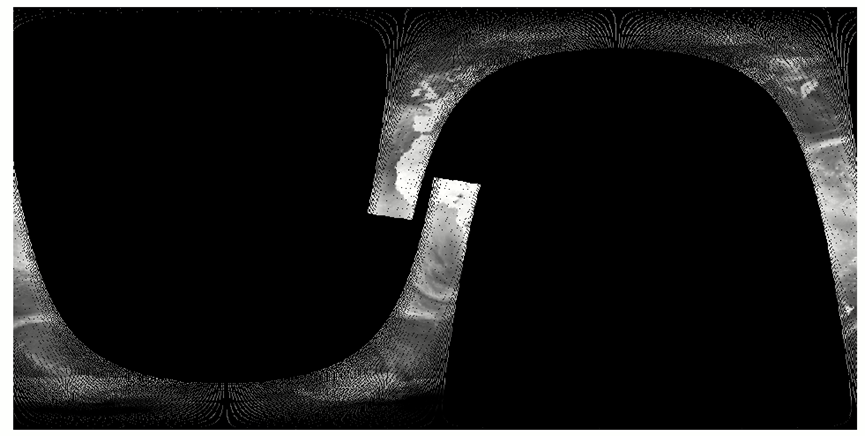
接着对套入的目标数组进行最近邻插值，如果没有进行插值，情况如下：

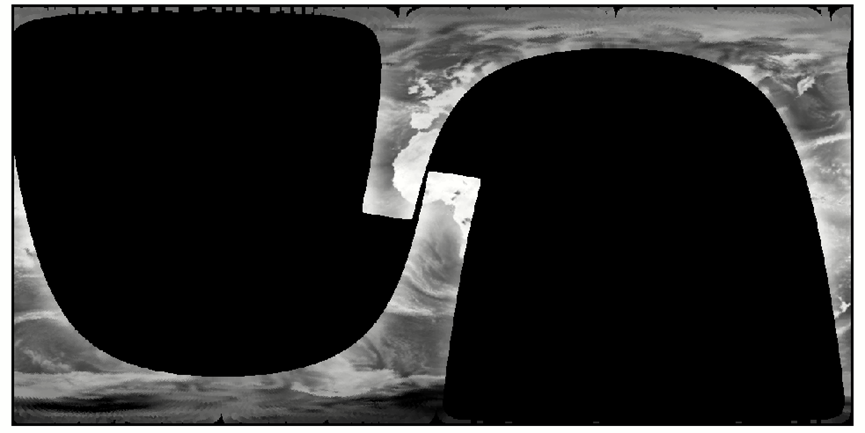
进行最近邻插值后（9*9窗口内的最近有效像元为填充值），结果如下：

但是由于数据集巨大，关于最近邻插值此处进行了注释，将该操作移至后面镶嵌操作之后，数据量大大减少，所花费时间成本也极大降低。

2 镶嵌和最近邻插值

2.1 镶嵌

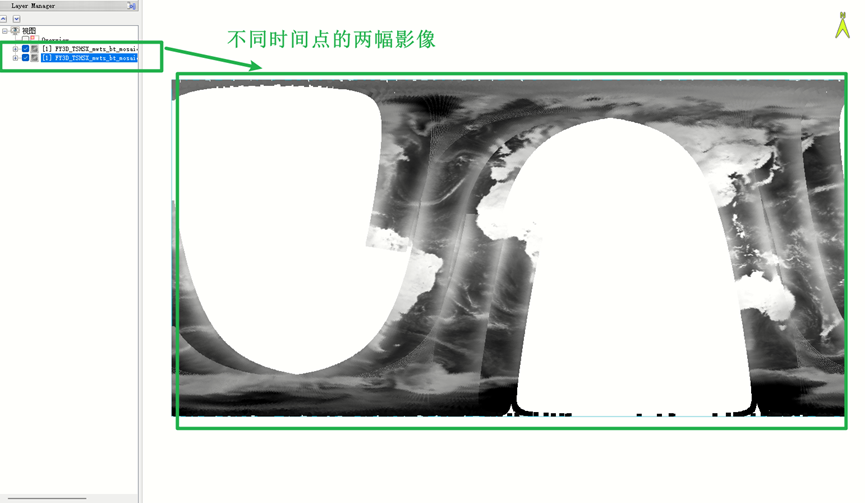
def img_mosaic(mosaic_paths: list, return_transform: bool = True, mode: str = 'last'):"""该函数用于对列表中的所有TIFF文件进行镶嵌:param mosaic_paths: 多个TIFF文件路径组成的字符串列表:param return_transform: 是否一同返回仿射变换:param mode: 镶嵌模式, 默认是Last(即如果有存在像元重叠, mosaic_paths中靠后影像的像元将覆盖其),可选: last, mean, max, min:return:"""# 获取镶嵌范围x_mins, x_maxs, y_mins, y_maxs = [], [], [], []for mosaic_path in mosaic_paths:ds = gdal.Open(mosaic_path)x_min, x_res, _, y_max, _, y_res_negative = ds.GetGeoTransform()x_size, y_size = ds.RasterXSize, ds.RasterYSizex_mins.append(x_min)x_maxs.append(x_min + x_size * x_res)y_mins.append(y_max+ y_size * y_res_negative)y_maxs.append(y_max)else:y_res = -y_res_negativeband_count = ds.RasterCountds = Nonex_min, x_max, y_min, y_max = min(x_mins), max(x_maxs), min(y_mins), max(y_maxs)# 镶嵌col = ceil((x_max - x_min) / x_res).astype(int)row = ceil((y_max - y_min) / y_res).astype(int)mosaic_imgs = []  # 用于存储各个影像for ix, mosaic_path in enumerate(mosaic_paths):mosaic_img = np.full((band_count, row, col), np.nan)  # 初始化ds = gdal.Open(mosaic_path)ds_bands = ds.ReadAsArray()# 计算当前镶嵌范围start_row = floor((y_max - (y_maxs[ix] - x_res / 2)) / y_res).astype(int)start_col = floor(((x_mins[ix] + x_res / 2) - x_min) / x_res).astype(int)end_row = (start_row + ds_bands.shape[1]).astype(int)end_col = (start_col + ds_bands.shape[2]).astype(int)mosaic_img[:, start_row:end_row, start_col:end_col] = ds_bandsmosaic_imgs.append(mosaic_img)# 判断镶嵌模式if mode == 'last':mosaic_img = mosaic_imgs[0].copy()for img in mosaic_imgs:mask = ~np.isnan(img)mosaic_img[mask] = img[mask]elif mode == 'mean':mosaic_imgs = np.asarray(mosaic_imgs)mask = np.isnan(mosaic_imgs)mosaic_img = np.ma.array(mosaic_imgs, mask=mask).mean(axis=0).filled(np.nan)elif mode == 'max':mosaic_imgs = np.asarray(mosaic_imgs)mask = np.isnan(mosaic_imgs)mosaic_img = np.ma.array(mosaic_imgs, mask=mask).max(axis=0).filled(np.nan)elif mode == 'min':mosaic_imgs = np.asarray(mosaic_imgs)mask = np.isnan(mosaic_imgs)mosaic_img = np.ma.array(mosaic_imgs, mask=mask).min(axis=0).filled(np.nan)else:raise ValueError('不支持的镶嵌模式: {}'.format(mode))if return_transform:return mosaic_img, [x_min, x_res, 0, y_max, 0, -y_res]return mosaic_img

这里的镶嵌不仅仅可以解决相同地理位置的镶嵌，也可以解决不同地理位置的拼接，拼接方式支持最大最小值计算、均值计算、Last等模式。
思路非常简单，就是将输入的每个数据集重新装入统一地理范围的箱子（数组）中，使所有数组的角点信息一致，然后基于数据集个数这一维度进行Mean、Max、Min等计算，得到镶嵌数组。

2.2 最近邻插值

def window_interp(arr, distances):if np.sum(~np.isnan(arr)) == 0:return np.nan# 距离最近的有效像元arr = arr.flatten()arr_sort = arr[np.argsort(distances)]if np.sum(~np.isnan(arr_sort)) == 0:return np.nanelse:return arr_sort[~np.isnan(arr_sort)][0]

思路与之前一致，不过重构为函数了。

具体代码见项目：https://github.com/ChaoQiezi/read_fy3d_tshs

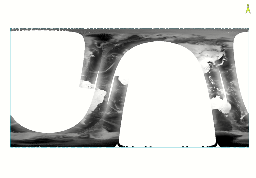
这是原始数据集：

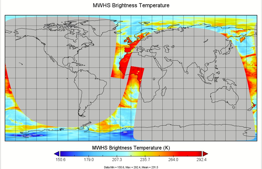
这是目标结果：